On the Nature of Hysteresis

I feel a deep understanding of the concept of "Hysteresis" is very important. When generally considered, this phenomena gives rise to losses seen in the dielectric of a capacitor or lamination of a transformer, these can be seen in the form of heat (emission of infrared photons). Alternatively it can remove work from a circuit without associated heat loss (a new form of loss not described in any common textbook), and oppositely impart work to the circuit from cooling of the environment surrounding the cicuit element (absorption of infrared photons).

Here's an interesting abstract of an article written by Mr. Dollard on this subject:



In the theoretical investigation of electric induction the propagating velocity of the transverse electro-magnetic (T.E.M.) component of induction is the only propagation constant considered. The propagation throughout space of the independent magnetic field of induction and the independent dielectric field of induction is not considered. In reality, however, these fields of induction start at the conductor and propagate from there throughout space at a definite velocity; that is, at any point in space the field of induction of magnetism or dielectricity at any moment in time corresponds not to the condition of induction at the conductor at that moment but that at a moment earlier by the time of propagation from the conductor to the point in space under consideration. Hence the given field of induction lags in time the more, the greater the distance from the conductor.

This lag in phase with respect to distance results in the cycle of energy return of the field of induction falling behind its point of phase opposition with the cycle of energy storage. This lag in phase gives rise to an energy component, that is an effective magnetic resistance or an effective dielectric conductance to the reactance or susceptance of the magnetic & dielectric fields respectively.

The phase angle of this lag in the cycle of energy return has been called the angle of hysteresis of the inductive medium and has become well known for ferrous materials. However, the application of this concept to the inductive medium known as the aether has received no attention except by Steinmetz. The purpose of this paper is the adaptation of Steinmetz' inductive propagation to the study of the hysteresis of the aether and a determination of the propagation velocity therefrom.

Going back to Heaviside's work, we have the H field or "intrinsic magnetization" and the B field or the "induced magnetization". H was considered the applied field and B the resultant field and hence the older term "magnetic induction" for B.

Heaviside points out that the B field and H field do NOT have to follow one another and usually do have a time lag between one another. This phenomena is generally called hysteresis, this HYSTERESIS is something that can consume (usually happens) or produce (rarely happens) electrical energy. Mr. Dollard has pointed this out here on the forum and in his published works, but it wasn't until recently that it all came together in my head.



A difficult but interesting read:
Oliver Heaviside - Forces, Stresses & Fluxes of Energy in the Electromagnetic Field [1891]
The above page 469 shown is from this article.

It would seem Heaviside inadvertently discovered the basis for the actions in which synchronous parametric variation may work, at least for the magnetic circuit. While he is talking about another subject its funny to read that and not think of parametric variation of an inductance.

Garrett M

On the Nature of Hysteresis

I feel a deep understanding of the concept of "Hysteresis" (the lagging of an effect behind its cause) is very important. When generally considered, this phenomena gives rise to losses seen in the dielectric of a capacitor or lamination of a transformer, these can be seen in the form of heat (emission of infrared photons). Alternatively it can remove work from a circuit without associated heat loss (a new form of loss not described in any common textbook), and oppositely impart work to the circuit from cooling of the environment surrounding the circuit element (absorption of infrared photons).

Here's an interesting abstract of an article written by Mr. Dollard on this subject:



In the theoretical investigation of electric induction the propagating velocity of the transverse electro-magnetic (T.E.M.) component of induction is the only propagation constant considered. The propagation throughout space of the independent magnetic field of induction and the independent dielectric field of induction is not considered. In reality, however, these fields of induction start at the conductor and propagate from there throughout space at a definite velocity; that is, at any point in space the field of induction of magnetism or dielectricity at any moment in time corresponds not to the condition of induction at the conductor at that moment but that at a moment earlier by the time of propagation from the conductor to the point in space under consideration. Hence the given field of induction lags in time the more, the greater the distance from the conductor.

This lag in phase with respect to distance results in the cycle of energy return of the field of induction falling behind its point of phase opposition with the cycle of energy storage. This lag in phase gives rise to an energy component, that is an effective magnetic resistance or an effective dielectric conductance to the reactance or susceptance of the magnetic & dielectric fields respectively.

The phase angle of this lag in the cycle of energy return has been called the angle of hysteresis of the inductive medium and has become well known for ferrous materials. However, the application of this concept to the inductive medium known as the aether has received no attention except by Steinmetz. The purpose of this paper is the adaptation of Steinmetz' inductive propagation to the study of the hysteresis of the aether and a determination of the propagation velocity therefrom.

[end of abstract]

Some follow-up reading to go along with the above article:

Eric P. Dollard, “Wireless Engineer”
The Transmission of Electricity, Part I, Sept-Oct 1987 JBR, pgs 4-7
The Transmission of Electricity, Part II, May-June 1988 JBR, pgs 10-12

Going back to Heaviside's work, we have the H field or "intrinsic magnetization" and the B field or the "induced magnetization". H was considered the applied field and B the resultant field and hence the older term "magnetic induction" for B.

Heaviside points out that the B field and H field do NOT have to follow one another and usually do have a time lag between one another. This phenomena is generally called hysteresis, and is something that can waste (usually happens) or impart (rarely happens) work to a circuit element, dependent upon the conditions present. Mr. Dollard has pointed this out here on the forum and in his published works, but it wasn't until recently that it all came together in my head.



A difficult but interesting read:
Oliver Heaviside - Forces, Stresses & Fluxes of Energy in the Electromagnetic Field [1891]
The above page 469 shown is from this article.

It would seem Heaviside inadvertently discovered a potential basis for the actions in which synchronous parametric variation may work, at least for the magnetic circuit. While he is talking about another subject its funny to read that and not think of parametric variation of an inductance.

Garrett M

JF Murray & Parameter Variation in Mechanaical Systems Pt1

Below are some interesting excerpts taken out of James F Murray's 1990 article New Concepts in Power Generation:

...Slowly I realized that in many cases Tesla was speaking about very rare or very different scientific phenomena with an attitude of complacency as if he felt that "surely everyone understands this basic material". But everyone did not understand. They were still struggling to digest Tesla's earlier concepts. Tesla did not trust most of his contemporaries. He never bothered to adjust his use of semantics to comply with accepted definitions. If he was misunderstood he was unconcerned. As a result, after many years this attitude eventually led to multiple interpretations of the meaning and intent of Tesla's work. His statements were considered enigmatic and eventually meaningful communication between himself and the scientific community ceased altogether. But Tesla continued expounding his discoveries as usual, unaware that the wisdom in his words fell upon deaf ears. Animated by the conviction that great knowledge had been lost, I set out to establish where Tesla had made his departure from recognized physics. Guiding myself by intuition, and by the implications hidden in various projects which he had proposed, I concluded the following:

A) There must be more than one kind of resonance and more than two kinds of induction supported by the laws of nature.
B) Tesla had discovered something very fundamental about the relationship between energy and power that still eludes the rest of the world.
C) Most of his later inventions, including the Magnifying Transmitter, probably made use of this "secret" knowledge, and therefore, still remain misunderstood by the scientific community as well as the general public.

...

Energy Resonance

I left Michigan not a moment too soon. My funds were gone, my hair was falling out, I had developed a bleeding ulcer, I was overweight and I couldn't sleep. I needed a complete overhaul. The company I was working for was good enough to transfer me to a small mining community in Eastern Pennsylvania. Once I had gotten established, I promptly joined the Y.M.C.A. where I began working out on a regular basis, and I found myself a lovely girlfriend. The last thing I wanted to do was to think about electricity! This attitude was short lived, however, for there were numerous electrical problems in the mind which I could not avoid and little by little I began thinking about my research again. The situation was completely different now though, because I had no shop and no equipment with which to experiment. Circumstances forced me to make my investigations mathematically. It seemed as if there were a million questions to answer and each would require rigorous mathematical analysis. With no models for generating data, my options were indeed limited. What I needed was to discover some underlying principle which could tie together all the loose ends and give direction to my research. But where do you look for something which no one else has found? Asking these questions seemed to prompt an answer “how about right under your nose”? True, the least obvious spot to hide something is right out in the open. Perhaps what I was looking for was so fundamental and so universal that no one suspected its existence. I began to ponder anew the most elementary of physical concepts: Force, Work, Velocity, Momentum, Newton's Laws and, of course, the Conservation of Energy. I was not interested in simply reviewing problems in physics, but rather in achieving a fresh point of view on principles which I had long ago taken for granted, and which I used almost daily through habit rather than by reason. To accomplish this end I began to apply differential and integral calculus to very basic equations in order better comprehend their origins and dimensionalities. I rambled through hundreds of calculations, and while I did greatly clarify many things in my own mind, I made no earth-shattering discoveries. However, eventually I came upon the basic relationship which links work to force and distance:

W=FS

This I differentiated with respect to time in order to develop an expression for power:

dW⁄dt=d(FS)⁄dt

Therefore,

dW⁄dt=F(dS⁄dt)

and...

Here I suddenly paused, when I realized that I was solving this derivative through habit and convenience. I had removed F from the parenthesis without thinking. How did I know that the force was constant? In many cases the force is actually a variable. So I started over:

W=FS

dW⁄dt=d(FS)⁄dt

Therefore,

dW⁄dt=F(dS⁄dt)+S(dF⁄dt)

and

P=Fv+S(dF⁄dt)

This equation states that if F is allowed to vary in time, then the power must consist of two components, Fv, the force times the velocity, and S(dF⁄dt), the distance times the rate of change of the force with respect to time. In other words, not only must the agency supplying the power pay for moving the force through a minute distance, dS in some minute time dt, but it must also pick up the tab for the changing forced dF⁄dt over the total distance S. I stared at the new relationship P=Fv+S(dF⁄dt) fully aware that something was going to happen. I kept thinking about the transforming generator, about the increased torque necessary to turn it and about the low conversion efficiency. But another part of my mind was trying to tell me something else. Something about non-linear rates of change, something about logarithmic functions, something about an equation in the fourth quadrant, something about the derivative of decreasing functions! Yes, the derivative of a decreasing function is a negative quantity! This means that if F were decreasing in time, then dF⁄dt would be negative, in which case:

P=Fv+(-S(dF⁄dt)) or P=Fv-S(dF⁄dt)

So if F decreases fast enough, then theoretically, dF⁄dt could become a large enough negative quantity to effect the magnitude of the positive power component such that if

P_1 = Fv and P_2 = Fv -S(dF⁄dt), then P_1 > P_2,

In which case, if P_2 represents power entering a system and P_1 represents power leaving the system, then the system would demonstrate a net power gain. But how could such a thing happen if energy must be conserved? It required three more years of mathematical study before I managed to isolate and demonstrate a simple mechanical system in which such an effect is apparent. And I am both proud and relieved to say that conservation of energy is not only upheld, but utilized extensively in my proofs. What does develop in a totally new light, however, is conservation of work. It has always been assumed that the work done must equal the change in the available energy under all circumstances. However, this proves to be true only in traditional linear systems! In non-linear systems, two additional conditions can be demonstrated:

I. The work done is greater than the change in available Energy.
II. The work done is less than the change in available Energy.


Below is an interesting excerpt taken out of James F Murray's 1983 article Introduction to the Concepts of Energy Resonance:

Power: Dissipative and Conservative

A great deal of confusion seems to arise among professionals and laymen alike when mention is made of the high efficiencies associated with the constant power systems of the Parametric variety. In conventional Power Systems, the number of independent variables is kept to an absolute minimum. An example of this can be found in modern Electrical Transmission networks, in which the only effective variable is the current. In sharp contrast to this situation, there can be many related variables in a parametric power system, each of which is phase locked one to the other, and all of which are synchronized to a common time base.

The word "parametric" apparently has no impact on the average mind, for immediately vehement arguments are advanced supporting the dissipative nature of all power systems and their limitations in accordance with the well-established laws of entropy. Additionally, the traditional defender will almost always be pleased to inform any inquiring novice that all known power systems have long ago been developed to their highest permissible levels of efficiency, and any notable improvement would represent a violation of the Second Law of Thermodynamics.

In rebuttal to such rigid attitudes, it is most important to realize that two types of work systems are known to the physicist. There is the non-conservative, or the dissipative, work function, which is responsible for the evolution of heat or any other non-recoverable energy form. And there is the conservative, or recoverable work function, which makes itself known by effecting a useful change in some other form of energy, such as kinetic, gravitational potential, or chemical, to itemize only a few.

Accordingly, then, there are also two types of power to consider: the dissipative form and the conservative form. It is the second type of power to which we must ultimately address our attention if we wish to gain an insight into the complexities of Parametric Physics. However, for the sake of ensuring continuity in the development of this theme, the dissipative power system shall be explained first.

Imagine a mass sliding down an inclined plane. The slope of this plane, and the frictional coefficient of its surface are such that
the mass m shall descend with a constant velocity v

Under these conditions, the force of gravity, acting upon the descending mass, shall develop a constant power over the entire course of the mass movement. This power shall represent the time rate of work done by the force of friction over the surface of the incline traversed by m.

The question now arises, however, what work can the force of friction do? Unfortunately, it can only generate heat, and heat is a dissipative agent. Therefore, although this hypothetical system can indeed produce a constant power over a designated interval, the type of power delivered is non-recoverable, and therefore, can serve no further use.

What then of the other form of power? How can its meaning be approached? Of what use is it, and under what conditions is it constant?

...

To be continued in part 2

Garrett M

JF Murray & Parameter Variation in Mechanaical Systems Pt2

Continuing from part 1, a few more exerpts from Introduction to the Concepts of Energy Resonance

...

Contemplation upon these results suggests an interpretation that may well lead to a general law long overlooked, or at least only partially understood:

"The conservative power developed in any system may be made to conform to the profile of any equation whatsoever, so long as that component of the developed velocity which is parallel to the natural line of action produced by the gradient in question is properly manipulated by the imposition of an appropriately distributed impedance."

Or, more simply stated, "The time structure of the Kinetic Energy developed in any system will be a function of the manner in which the gradient is deployed with respect to the displacement, and the power evolved will be the rate of change of this function."

In accordance with this postulate just advanced, an answer to the question posed earlier may now be ventured: "The circumstance in which constant power can manifest in a system undergoing an acceleration will be found in any arrangement which provides for the development of a constant velocity component by the body traversing the gradient, such that the mass will drop through portions of the gradient having equivalent potentials in equal periods of time".

Linear Energy and Energy Resonance

Dwelling on the realization that the instantaneous power is a derivative of the Energy Function in any system, it becomes clear that, if the conservative power is constant in a given application, then the energy which gives rise to it must, of necessity, be represented by a linear equation. And if the energy is represented by a linear equation, then its amplitude must build in discreet steps which increase according to even integer proportions such as 1, 2, 3, 4, 5, 6, etc. Here, then, resides the most important qualification for describing a Parametric Energy System; the energy must be structured in time; it must be quantified!

No one should be surprised at this statement, for there is no reason why certain of the principles inherent in quantum mechanics of particles should not be applicable to macroscopic systems as well. However, because total parity has not yet been proven between these two systems, hereinafter the term Linear Energy rather than Quantized Energy, will be used to further descriptions of the energy in Parametric Systems.

Before proceeding with the development of further concepts associated with Linear Energy Systems, it is imperative that one basic precept be well understood.

What is perhaps most crucial, and most confusing, is the notion of a constant velocity component in an accelerating system.

A little reflection on this situation will yield the fact that the motion in question here cannot be rectilinear, but must obviously be a compound form of motion, having components on at least two axis systems.

It can be hypothesized, then, that the motion under study must, of necessity, represent some form of angular velocity, one component of which remains constant in magnitude. If the vertical velocity component, vy, is assigned this fixed character, then vyt will represent the vertical displacement over the elapsed time, or the height dropped through. Accordingly, then, the product of the vertical velocity component and the time defines the relationship between a "quantum" of Potential Energy and a "quantum" of Kinetic Energy in a Linear Energy System. This is demonstrated in the following derivation:

...

Note that the power must be a constant as it is the product of two other constants.

It should be obvious at this point that in order to ensure the production of constant power over the entire range available in the gradient, two requirements must be met and upheld. First of all, the body in question must drop through equal segments of potential in equal periods of time. This ensures that the change in Potential Energy with respect to time is linear. Secondly, the applied force must decrease while the displacement increases as a function of the acquired velocity. These conditions ensure that the change in the Kinetic Energy with respect to time is also linear.

In order to fulfill these requirements, the gradient must be "structured" in a very specific manner. An "impedance" therefore must be "imposed" upon the gradient to distribute its effects in space and time, such that the acquired energy will be linear and the developed power constant.

In the realm of simple mechanics, an inclined plane represents an impedance imposed on the gravitational gradient. However, the effects of such an impedance upon the acquired energy were discussed previously, and the results were certainly not linear.

In order to design an adequate impedance for linearizing the energy extracted from the gravitational gradient, it is only necessary to compute the x and y coordinates traced out by a particle moving according to such a law that the square of each instantaneous value of its velocity is made to yield a line of constant slope when plotted with respect to time. Such is the case for the expression

...

The utilization of these formulas and the classical relationship describing angular motion give rise, now, to a considerable volume of new information after a few simple calculations. If these results were charted, a study of the graphs would quickly reveal the fact that all of the plots except for those exhibiting the angular work, and the angular power, are nonlinear. This gives rise to a thought worthy of consideration. Apparently, linear parameters develop non-linear energy curves, while non-linear parameters seem to be responsible for the evolution of linear energy curves. This suggests the development of interesting, but complicated, scaling problems in the engineering of Linear Energy Systems. It may also explain why effects of this kind have never been stumbled upon; the designer must know exactly what he is doing!

If it were possible for you to mentally observe the behavior of the moment of inertia in this system, you would notice the steady and continual change in the length of the radius vector over each interval. The rate of change of r with respect to t must be precisely determined and controlled, such that the dynamic change in the moment of inertia, first retards the acceleration, and then, when required, assists it, but in such a manner as to insure that the product of the instantaneous torque and the instantaneous angular velocity are always equal to some predetermined constant, and the time interval between each event is the same.

Because each separate interval is equal in time, the total time is a cyclic constant. Here, then, lies the true meaning of the elusive concept of the dynamic constant, otherwise known as the phenomenon of constant period!

Further reflection on these concepts will disclose facts even more incredible! The angular velocity may be represented in terms of a frequency f:

ω=2πf

Hence, the frequency is simply

f=ω⁄2π

Because 2π is a constant, the frequency is seen to be in direct proportion to the angular velocity. However, this presents an information conflict in terms of classical theory. How can the period be constant if the frequency is changing in time and phase?

The answer to this apparent contradiction lies in the fact that the combined energies contained in each instantaneous frequency sum together in quantum increments with the passage of time. In this way, each frequency involved contributes to the total volume of energy in the system and, theoretically, the total of quantity of the available energy can increase linearly without bound! Thus, the energy has been made to resonate! This is the true meaning of Linearized Energy! And it is now understood that the constant period is the reciprocal of the overage frequency.

It is important to understand that this process is diametrically opposite to Frequency Resonance. For when a particular frequency is made resonant, the system parameters are adjusted so as to maximize the amplitude of the fundamental wave in question and suppress all other frequencies and harmonies to some ineffective level. In doing this, however, more than 36.4% of the energy which could have been made available for use is discarded!

The correct integration of all this data is essential to gaining insight into the unusual operation of Resonant Energy Systems. It must be understood that the incoming power flow is made to become constant in time, thus the energy simply continues to accumulate linearly. Here, then, lies the mechanism which provides the efficiency advantage associated with Resonant Energy: the primary source never delivers energy directly to a dissipative load, but rather to an energy storage system which then, over the second half cycle, delivers its accumulated energy to the load at hand.


References:
James F Murray,
New Concepts in Power Generation, JBR Vol. 46, No. 2, March-April 1990
and
Introduction to the Concepts of Energy Resonance, 2nd International Symposium on Unconventional Energy Technology, September 1983, Atlanta Georgia

Garrett M

Hey Garrett,

Thanks for starting this thread. I do not plan on becoming too active in discussion since I have experiments to run but figured that I would show some promising results regarding parameter variation. I have built a machine that consists of two alternators and a prime mover. The alternators are spinning at a ratio of 1:2 to give me a primary frequency and the 2nd harmonic of that frequency as per the instructions of Manelstam & Papalex, E.P. Dollard, and Steinmetz.

I am only using junk parts for my magnetic amplifier. It consists of laminations carefully chiseled away from a microwave oven transformer to equal roughly the same density as the iron in my alternator. The power windings of the magamp have been matched to the copper for a single phase in the alternator.

When I modulate the inductance of the magamp's power winding at the correct phase angle via the control winding, I get a waveform that looks like this:


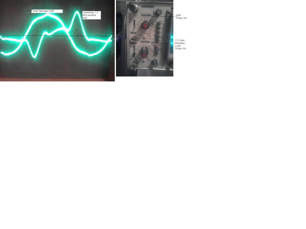
Sorry about the small picture but I don't have time to go back and make it better.

Notice the positive power (Ei) relations versus the negative power (-Ei) relations. They seem to be of approximately the same as far as the energy storage and the energy return goes. The noteworthy component is the 1.5 ohms worth of resistance that the current is "flowing" thru each time, lighting the car headlamp to a brightness that I don't like to stare at. This is all being done for 13 watts worth of modulation from the 2nd harmonic wave which has much more room for increases in efficiencies.

By no means have I analyzed this as extensively as one would need to for a thorough scientific analysis, but it sure is interesting to see the beginnings of what has been proposed by the pioneers.



Dave

Diferential & Integral Calculus and Other Thoughts

I want to point out a few things that might assist anyone who reads Jim Murray's work or the citations I just posted. He is talking about and implying concepts of differential and integral calculus the WHOLE TIME.

For the non math savvy, in calculus you generally deal with two distinct plots (i.e. curves or graphs) one plot (differentiation) could be speed v(t) as seen on a "speedometer" (instantaneous value of speed) and the other (integration) distance f(t) as seen on the "odometer" or "trip meter" (total distance traveled). For an excellent book on calculus and some video help on calculus, Professor Strang of MIT has done a great job on the MIT OCW (open course ware) with his non-formal instructional lectures, "Highlights of Calculus" , along with giving free access to his 1991 book "Calculus" (the link i gave is a higher quality version of the book, the one from MIT was deliberately molested to make you want to buy the second edition). Alternatively you could go to "Khan Academy" and watch a few videos there on single variable calculus for a refresher.

Dave,

What I find very interesting in your demonstration, is that the MMF waveform, during the "spike portion", is always in opposition of the applied EMF, that would imply that you are having a reversal in the power factor or a PF of +1 abruptly changing to a PF of -1 during a portion of the waveform period, presumably during the modulation of inductance from the MagAmp. That of course is if the probes are connected correctly, if you were to flip the orientation of the oscilloscope probes it would invert the waveform. BUT it would seem that the MMF, before the modulation of inductance takes place, going through the 1.5ohm resistor is mostly in phase with the EMF with a slight phase shift from the small relative inductance of state L0, this would imply that the probes are connected properly. An interesting experiment to perform, would be to try to remove work from the system, by modulating to a maximum inductance when MMF is at its lowest and reduce the inductance to a minimum when the MMF is at its maximum. This would show you that the circuit is working as well, but in a bizarre state of loss of work that is conventionally uncountable for. Something else to look for is the quantity of heating or cooling of the iron core of the MagAmp.

I have a few questions if you would like to answer them. One, how are you modulating the inductance of the MagAmp, more specifically what type of waveform are you using and what is (if you want to divulge) the design of the MagAmp magnetic circuit structure.

I might be able to lend some assistance in your design if your interested. Personally I have found a square wave control signal to be very UNNATURAL and to cause lots of EMI noise. Subsequently a sine wave gives much more natural power waveforms.

Furthermore the excerpts I posted of Jim Murray's 1990 & 1983 articles are VERY VERY important to read. Convert all the mechanical analogies he gives to terms of electrical circuits and you will see some amazing insight into your experiment. Knowledge of calculus is highly recommended in grasping what he means by "constant", "linear" and "nonlinear", remember there are always two plots, differentiation and integration, the relationship of the two is what he is referring to.

...

On a side topic, I think I finally grasp what Mr. Dollard is talking about when referring to the ELECTRIC FIELD. From what I now understand, the electric field could be considered as the Poynting Vector "S" having a flux Q in "planks". Much like the Dielectric Field has G (aka E), intrinsic dielectric field gradient, & D, the induced dielectric field caused from polarization, both creating a flux "psi" in columns. The Magnetic Field has H, intrinsic magnetic field gradient, & B, the induced magnetic field caused from magnetization, both creating a flux "phi" in webers. The multiplication of G & H or D & B (or both sets) produces the "Poynting" vector S or electromagnetic "energy flux" Q of the Electric Field. An excellent read on usage of the Poynting Vector in Lumped Circuit design (only a preview) is Electromagnetic Modelling of Power Electronic Converters By J. A. Ferreira. An interesting topic that would go along with the Poynting Vector is that of the supposed "Heaviside Flow" (shall we call it Vector O, for Oliver) that Tom Bearden purports. This is the "curled" "energy" that doesn't diverge into a wire for use whereas the Poyting Flow is exactly that which diverges into the wire. This being the "useful" "electromagnetic energy" we use today, while supposedly there is a huge flow of unusable "energy" present in the form of the "Heaviside Flow".

Some food for thought.

Garrett M

Obviously my response is in red. I just finished a new control winding of twice the number of turns as well as a bigger wire gauge so I am about to see what happens when I get more magnetism into the control winding. I have a feeling that this material is crap for this type of work because I plotted the inductance versus the control winding ampere turns and it never quite fully saturates as Mr. Dollard suggested.

Dave

Parameter Variation Prelude

I have recently started doing some research into parameter variation again and have had some encouraging experimental results. Also, I have gotten a lot of it written down and edited for sharing here on the forum.

For those who are interested in this subject, the title of my future post will be:

Angle of Hysteresis & the Continuity of Energy;
An exploration into the Synthesis of Energy via Parameter Modulation

It won't be ready to post for a week or two (still lots of editing to do), but here's an abstract, some graphs and a few quotes to keep you interested:

Abstract

When working with parameter modulation, asymmetric distortions in the systems power waveform, due to the angle of hysteresis of induced fields to intrinsic fields, causes the appearance and disappearance of electrical energy. This is seen in the form of an artificial shunt conductance or an artificial series resistance, these artificial quantities can be found to have negative values when certain angles of hysteresis are observed, causing an increase of energy per half cycle into the electrical system, while the opposite causes a decrease of energy. A basic theory to define these artificial quantities along with negative parameter values (such as negative inductance and negative capacitance) will be discussed and referenced with known electrical systems that exhibit the phenomena.

*Tech Note, synchronous motors are also sometimes called "synchronous condensers" or "rotary condensers", because they have a leading current in certain situations like a condenser or capacitor would. This causes them to appear as a NEGATIVE inductance to the circuit in which they are used. The negative inductance property of an over excited synchronous motor is commonly used to cancel the reactance of "positive" inductive loads (induction motors and transformers) and thus restoring a unity power factor. Much like how a capacitor stabilizes a DC circuit, a synchronous motor can stabilize an AC circuit by storing energy in the form of mechanical mass as a motor and returning that energy back to the circuit through generator action.

Below is a reactance plot showing the action of negative and positive reactive circuit elements:


A quote from what Tom Brown had written regarding Mr. Dollard's work:

"The Alternating Electric Waves paper, presenting Eric's Four Quadrant Theory of Electricity, was written after his discovery of how to generate excess magnetizing power in an industrial situation (using synchronous motors in a huge shipyard) and make the KVAR (Kilo Volt Amperes Reactive) meter turn backwards. Eric discovered that these industrial meters are pinned so that they will not turn backwards, but they can be stopped, creating readily realizable savings for the industrialist."

From Steinmetz's chapter on Reactance Machines:




A step and sinusoidal variation of reactance:



Also, the much need topic of energy movement will tentatively be brought into discussion:


More to come after I finish editing,
Garrett M

Hey Garrett,

Recently, I purchased a digital storage oscilloscope that has waveform math functions and an xy display for use in determining the BH curve of the material in use. With this new equipment, it is much easier to determine what is going on in the circuit. I have revisited harmonic modulation and have been able to get some really good looking waveforms. However, I'm going out of town for a few days and won't be able to get anything posted on it until I get back. The only suggestion that I have to experimenters is to use a material with a highly square hysteresis loop and the power windings must be of a high magnification factor(ratio of energy stored to energy dissipated).

Good luck,

Dave

P.S. Thanks for always taking the time to post everything in a very clear and organized manner. I don't have that kind of patience unless somebody is asking me for clarification.

Synthesis of Electrical Energy Via Parameter Variation Pt1

Thanks for the notes Dave, looking forward to seeing your collected data and experimental results. Here's a very meager and simple demonstration of the principle using the mode of natural excitation.

Introduction

I performed a very basic experiment in the "generation" of electrical energy via parameter change last night that proves the 1930s theory of the original Russian investigators:

L Mandelstam
N Papalexi
A Andronow
C Chaikin
N Minosrsky

Whom of which, I have read every available English copy of their written works. These gentlemen have laid out a rigorous scientific foundation for the generation of electrical oscillations via parameter variation, with their concise and lucid writings.

The Experiment

The magnetic circuit for the experiment came from a series-wound brushed two-pole AC motor,



confiscated from a defunct vacuum cleaner, which had already had the rotor windings removed and machined to look like a wide rectangle as opposed to its original cylindrical shape. Thus giving the rotating magnetic element differing degrees of reluctance and thus periodic changes in attractive force which made the motor move when tightly timed control pulses were administered. This constituted a prototype pulsed DC reluctance motor that I made some time ago. Maximum rotational speed was ~4.2k RPM.







It just so happened that this rotor structure served as a time varying inductance, therefore I simply unhooked all the electronic controls to the motor and mechanically coupled a separate DC motor to the reluctance motor,



I then connected two 30 micro-Farad capacitors in shunt with the series connected two pole reluctance motor hooked up a Simpson milli-wattmeter (confiscated from a defunct HP bolometer) (*I didn't expect it to produce very much power) a sensitive current clamp and a 1x configured oscilloscope probe to the LC tank circuit for measurement. A 150MHz digital scope, with both inputs set to 1x, 5mV and 500mV per graticule respectively for channel 1 (current probe) and 2 (voltage probe), was used to take the below oscillogram,



Tech Note, the "spikes" seen in the current waveform are not real, they are induced into the current clamp by the brushed DC motor arcing, this is a common problem for brushed magnetic circuits. Hence they are only an "artifact" and do not represent any meaningful information other than the rotational rate of the motor. A solution to this annoying problem is an "rC snubber" shunted across the motor terminals to suppress the spark and oscillations incurred by the brushes. An alternate solution is to place an earthed electrostatic shield around the current clamp.

We get two values for current and voltage due to a compound wave having two different periods from double resonance (f_max=263cps f_min=208cps):

Current clamp was set to 100mV/A thus for channel 1, we take the voltage in mV and divide by 100mV to get the current in amperes.
At f_max, 14mV/100mV = 0.140A peek
At f_min, 12mV/100mV = 0.120A peek

Voltage probe was set to 1x, oscilloscope was set to 1x, thus for channel 2 to get the voltage in volts we take the mV of oscillogram and divide by 1, or more simply its already proportioned.
At f_max, 1.7V peek
At f_min, 1.2V peek

The vector power oscillating in the system is given as Volt-Amperes, thus
At f_max, 0.238VA peek
At f_min, 0.144VA peek

Tech Note, The oscillation zero crossings and 1/4th / 3/4th periods do not directly line up with the maxima and minima of inductance change, they actually line up with the effective or average value, L_avg. This becomes a very important characteristic when examining the collected information. Curiously, the oscillatory node maxima for the current waveform are not at the 1/4th and 3/4th period locations as would be seen in a normal LC tank, i.e. they don't line up with the voltage zero crossings. The node maxima for voltage, however was aligned closely with the 1/4th and 3/4th periods, or the zero crossings of current. The current node maxima are offset due to parameter changes from the modulated inductance. Since a variable capacitor wasn't present, it makes sense that the voltage node maxima weren't materially changed.

This was at the resonant frequency of the time variant LC circuit, 232cps. At this point the milli-wattmeter was pegged, thus output in real power was greater than one milli-watt. It should be pointed out that this was a DC milli-wattmeter, therefore a rectifying bridge was used to connect the meter to the circuit. With the low voltage of the oscillatory circuit and the high Vf of the silicon bridge diode (~1.1Vf) this is only a qualitative measurement and not a quantitative measurement. It was useful, however, to find the exact resonant frequency.

Tech Note, to improve sensitivity of the watt meter, the Vf of the diode can be mitigated with a "DC block" capacitor and some DC bias, that way the bridge diode will pass and rectify the previously "clipped" portion of the AC wave giving more accurate results.



Interpretation of Collected Data

Circuit measurements done before experiment, LC with a BK 879b LCR meter @120cps and DC r with a Fluke 289 on “low ohm”, both meters were "zeroed" with used connecting leads before measurements:

Tech Note, all storage element measurements should be done at the working frequency seen when operating, since I didn't know what frequency it was going to be operating at and my LCR meter is a POS limited to 100, 120, 1k 10k cps, I used 120cps as a reasonable guess. which worked out okay for this experiment. However, all storage parameter effective values change with increasing or decreasing frequency, thus, measured values are only useful at a specific operating frequency or a very limited range of frequencies.

Variable Inductance:




Delta L, total relative change in inductance magnitude:



For given conditions, total relative change in inductance was found to be L_delta = 4.18mH

However, the effective relative change in inductance was found to be (L_delta)/2 = 2.09mH

Effective Depth of Modulation m, percent change in inductance magnitude:



For given conditions, effective depth of modulation m for inductive element was found to be, m = 30.02%

Static Capacitance:


DC resistance of inductor and connecting leads:


Continued in part 2.

Synthesis of Electrical Energy Via Parameter Variation Pt2

Equivalent Circuit Diagram (coil resistance not shown):



Inductance was effectively modulated 30.02% four times per revolution of reluctance motor with an effective delta L of 2.09mH per 1/4th rotation. If the inductance parameter changed 4 times for every mechanical revolution, the electrical oscillations per theory have to be at 1/2 this rate. Therefore, a 1:4:2 ratio of distinct rotations are seen in the system. 1 mechanical rotation = 4 parameter rotations = 2 electrical rotations.

Speed of DC Motor:



At 232cps or electrical rotations, the coupled DC motor rotated at one half this rate or 6960 RPM.

Here is another oscillogram showing the induced current from parameter modulation and the control signal from the timing wheel I had attached for use as a pulsed reluctance motor, which helped immensely in making clear what was going on.



Tech Note, each pulse is mechanically spaced 180°, three pulses mechanical represent 360°. As can be seen, one electrical wave fits between each pulse, thus one wave is produced for each half rotation and two electrical waves are produced for one full rotation.

Calculated frequency and half periods (with 0.76 DC-ohms):

L_max = 8.42mH, C = 59.18uF:




L_min = 4.24mH, C = 59.18uF:




L_avg = 6.33mH C = 59.18uF:




Measured frequency and half periods, due to hysteretic resistance:










The resultant measured frequency of 232cps, is at odds with the calculated 271cps LCR circuit (the "dc resistance" was included in the calculated measurement). This result reveals that there is a time variant resistance seen in the circuit due to hysteresis losses of the magnetic and dielectric elements and at very high frequencies, the AC resistance of connecting wires.

Continued in part 3

Synthesis of Electrical Energy Via Parameter Variation Pt3

Effective Hysteretic Resistance h:

The solution for finding the time variant resistance or artificial resistance can be found by reverse solving the expression for oscillatory frequency.



Since we are dealing with a compound wave, we need to reverse solve this equation twice for both natural oscillatory frequencies.



Two solutions exist for h_1:





Two solutions exist for h_2:



Mathematically considered, negative quantities are an actual possibility, thus the reason values for -h were listed. I would be thrilled if Mr. Dollard had something to say about this, but I doubt he will give a response to this post. I have some thoughts on this result, but will keep them to my self for now, as I am not confident enough on the accuracy of my conclusions.

Thus the total effective resistance of the circuit:



For the circuit in question, total effective resistance R = 9.305 Ω

The effective resonant frequency is:



For the circuit in question, effective resonant frequency f_osc0 = 232 cps

It should be pointed out, that there are an unlimited number of resonant points in this type of system. Due to the arbitrary value of the static storage element, in my case it was a parallel bank of 2 30uF capacitors. However, there will only be a limited number of static storage element values that derive a LARGE resonant oscillation, this is the ultimate problem of this type of circuit, I substituted many different values to get the largest oscillation which is seen in the oscillogram given earlier. I have some books coming on non-linear oscillations, maybe after a few weeks of reading, I'm pretty dense when it comes to absorbing new information, I will be able to give a solution to this very important problem.

Furthermore, the only way to avoid the compounded two-period wave, is to have a time variant capacitance (spring) to go with the time variant inductance (mass). That or a switched capacitor would solve the problem of a compounded two-period wave. Which may be desirable for certain applications and may very well lead to a larger resonant oscillation in the circuit, but, will remain un-experimented with for now. This reasoning is derived from the fact that we are operating outside of both resonant conditions calculated for the circuit. If only one mode of resonant exchange existed, and the circuit was operated inside of that mode, it would seem that the oscillations incurred would be greater than having two modes present and operating outside of both of them.

Tech Note 1, there are multiple modes of excitation for parametric systems, the mode used in this experiment was natural excitation. This requires a conjugate energy storage medium, in this case a capacitor, and whereby no power is already flowing through the system and all power provided was due solely to parameter variation. Mr. Murray, however, shows that an alternate mode exists when used in conjunction with a system that has a circulation or transfer of energy already taking place, by varying the parameter within the limits set by the "host" systems natural oscillatory rate. Curiously, in this condition NO conjugate storage medium is needed. Over excited synchronous motors already do this with AC power systems.

Tech Note 2, the magnitude of the current and voltage vectors of the oscillatory system given in this series of posts could have been assisted with a vacuum tube or transistor circuit adding gain into the system. This would be seen as a negative resistance used to cancel the natural and artificial losses of the oscillatory system. This is useful to find the maximum amplitude of oscillation possible, this idea is brought up in the book "Theory of Oscillations" by A Andronow & C Chaikin, 1949.

*The Curious Case of Confusion

I originally thought that I used the invert function on my oscilloscope to adjust the waveform to proper representation, however, this has now been found to not be the case. The waveform as seen in the first oscillogram in Pt1 was actually drawn correctly. I tested the circuit with a direct current to check that the current and voltage traces moved in the same direction on the scope and after playing around for 30 minutes or so, I concluded that they were in proper polarity.

Below, are two more oscillograms. They have different values from the one shown in Pt1 because the watt-meter was disconnected and the current waveform was cleaned up by placing an electrostatic shield around the current clamp and an rC snubber on the DC motor.

For no-load circuit conditions:

Average Frequency = 245.1 cps
Average Total Period = 4080 μS

High Frequency = 268.8 cps
Short Half Period = 1860 μS

Low Frequency = 225.2 cps
Long Half Period = 2220 μS

Total Effective Resistance = 6.91 Ω

*This is the correct and triple checked oscillogram of the circuit in operation. As can be seen it is the same as the one given in Pt1, but with higher peek values due to the watt-meter not being hooked up.



*This is the incorrect oscillogram. Due to the oddity of the waveform generated, I thought I had hooked up a probe backwards, so I captured this oscillogram as a correction, but this was NOT the case.



Conclusion

While the experiment didn't provide all that much electrical output, I am confident enough to say that this is a potentially viable solution to the worlds "energy crisis", or more aptly the worlds "intelligence crisis".

The amount of mechanical energy needed to turn the shaft is almost entirely INDEPENDENT to the electrical output. This was determined by applying a direct current of 10 amperes, well above the operating current of the coil, and using the same DC motor to drive the rotor. The results were found to have negligible effect on power draw of the DC motor. Next an alternating current of 4 amperes RMS (max I was able to provide) was administered in the same manner, the effect being even less than that of the DC, when the DC was lowered to the same effective value of the alternating current.

Concluding, it isn't mechanical energy that is being converted, but merely the rate of change in inductance or any other storage parameter. Thus you can assume that if you derived a method to change a storage parameter's value with minimal effort or exerted force, you would certainly have a system develop a COP well above unity.

The mechanical circuit equivalent is a changing mass for a mass-spring oscillator. If you were to increase the mass on the fall and lower the mass on the rise of the mechanical oscillatory period, you would exhibit negative resistance (due to gravity) and self sustained oscillations. The only energy required is that of changing the mass, which would take quite some ingenuity to resolve. If the energy exerted to change the mass is less than the energy imparted by gravity to the mass, you would have a COP greater than unity for a mechanical system.

The underlying principle of parameter variation is universal to all fields of science involving the movement of energy through time-variant storage elements, and is not limited to just electrical circuits.

Next up, when I get around to it, will be how to calculate for any arbitrary amount of electrical power to be generated by a parametric system with losses and other problems included, this however, will not be any time soon.

Food for thought,
Garrett M

Just wanted to pop in here and say that I will be coming back on-line next week and be able to contribute to this as well. The effect of negative resistance is of course as old as tubes.

There seems to be more than one way to "skin the cat" as they say. The capacitive plate and coil transformer setup I was working on has been producing very strange results and in digging into more texts and research I got to thinking about the ground side of the circuit, the plates either induce a negative resistance into the coil or the field induced within the self oscillation of the coil is the negative resistance, whats truly strange is that it's a passive component and thus a no-no from conventional theory.

look into tube design and negative resistance, I'll get some titles together in a bit and post them up.

Reluctance Motor Update

I have lots of new information regarding the reluctance motor as a modulated inductance. I still need some more time in "digitizing" the collected data and observances, a lot of good has come from this little experiment and a lot of confusing results as well. For a short update on the matter, the naturally excited circuit is basically an LCR circuit with a negative resistance as the driving source. The maximum resistive load that will still allow for oscillation, is equal to the source negative resistance subtract the inherent losses due to hysteresis, foucault (eddy) currents, ect. The addition of a load de-tunes the circuit, but not too much if it doesn't exceed the maximum. This mode isn't the most efficient for power generation, but lots of valuable information has been collected that would help describe other modes of operation.

As a heads up for those who care, my post on "The Angle of Hysteresis and Continuity of Energy" will be delayed due recent experimentation and may not be ready for a month or two, due to all the new information I have collected. Which is a good thing, it should be more comprehensive.

I think this project will eventually lead to some mathematical expressions that will actually provide an engineer-able device with an over-unity COP, that doesn't require strange/exotic theories, expensive materials or complicated ideas.

-------------------------------------

Madhatter,

Thanks for the comments on negative resistance. I have been looking into this phenomena for a while now and have come to some interesting but probably obvious conclusions on the subject, but will wait to post anything until I can confirm my thoughts or at least get a good hunch that I'm close to an acceptable explanation.

Garrett M